How to select projects and allocate funds to obtain the total maximum profit for facing many different investment projects in the production strategy management plan of discrete production enterprise

Bao Gang
ORCID iD:0009-0008-5357-9198
University of Ruse “Angel Kanchev”, Bulgaria

Pavel Vitliemov
ORCID iD:0000-0002-1747-7994
Web of Science Researcher ID: H-5795-2018
University of Ruse “Angel Kanchev”, Bulgaria

https://doi.org/10.53656/adpe-2025.18

PDF

Pages 197-216

Abstract. The market is developing rapidly, and the choice of production investment projects presents diversity and complexity. Manufacturing enterprises not only need to select high-profit target products (multiple target products) suitable for their own production but also need to reasonably allocate limited resources to ultimately obtain the maximum total income of all investment projects. Therefore, manufacturing enterprises are faced with many challenges when selecting production investment projects and allocating limited resources. In the process of selection and allocation, enterprises need to combine their own conditions to select investment and production, strengthen cost management, and pursue the maximization of investment benefits. Here, our research in this area becomes important.

This paper proposes a new method to establish an efficient process of investment project selection and resource allocation to obtain maximum total profit and emphasizes the importance of investment project selection and limited resource allocation. The basic steps and modules required for this process are described: the first step is to use the clustering analysis method (K-means) to cluster and screen the products with a high target profit in the market. In the second step, TOPSIS method is used in combination with the limited actual production conditions of the manufacturing enterprise to optimize the sequence of alternative and ideal solutions for the high-net profit products selected by the first step, and the good and bad solutions are sorted. The third step uses the dynamic programming model to optimize the allocation of resources for several target projects selected in the first two steps to obtain the total maximum profit. These 3 steps will be connected through MATLAB software series commands.

In this paper, theoretical analysis and software programming simulation are carried out to determine the effectiveness and feasibility of the scheme. The advantage of this system is to efficiently screen out high-net profit investment and production projects from many products in the sales market, sort and select the final target projects in combination with the actual production conditions and capabilities of the manufacturing enterprises themselves and rationally allocate limited resources to obtain the maximum profit return of the total investment. This is an investment process with goals and plans, reasonable screening and allocation as well as maximum return on investment.

Keywords: production investment; K-means clustering analysis; TOPSIS method; dynamic programming; screening and allocation; maximum return on investment

 

1. Introduction

The investment and return of production has always been the focus of manufacturing enterprises. The selection and investment of successful production projects can help enterprises obtain high profit returns, which is the basis for manufacturing enterprises to continue to operate better.

But in the actual process, how to find the production investment products and projects that are most suitable for their own production conditions and capabilities in the highly competitive market? This is an important problem that has been plaguing many manufacturing enterprises. If the enterprise finds the most suitable production investment project with high net profit, it can help the manufacturing enterprise to give full play to its own advantages and rationally allocate limited resources to obtain the maximum profit return. If the production investment project selected by the enterprise is not fully in line with the production situation of the enterprise or the investment fails, it will not only waste the resources and time of the enterprise, but also may cause the investment funds to fail to return to the enterprise on time due to the investment failure, the capital chain of the enterprise is broken, and the manufacturing enterprises are heavily indebted and eventually go bankrupt. So, the current research in this field is particularly important. However, most of the existing similar literature studies mainly focus on artificial intelligence or big data analysis on a relative range of past data or use a single model or method to analyze and forecast data and processes, which has certain limitations. Manufacturing enterprises need to expand the market to face a broader market for efficient screening. Enterprises should make use of their own production conditions and limited resources to challenge the possibility of more production investment to obtain the maximum return on investment profit. We seek a more concrete and effective approach.

This paper presents a qualitative research method by using model combination for selecting production investment projects, sorting target schemes and selecting the best target schemes, allocating limited resources reasonably. Through the establishment of a combined mathematical model or theoretical model to describe the specific problem, show its working principle and process, while using MATLAB software to demonstrate the solution.

The main goal of this paper is to help manufacturing enterprises in the production strategic management plan for facing of a large number of different production investment projects to carry out high net profit production investment products and projects sorting alternatives and ideal schemes and select target schemes reasonable allocation of limited resources and obtain the maximum profit. This process solves the problems of subjective blind investment production, unreasonable allocation of limited resources and low return on investment of manufacturing enterprises.

2. Concept of proposed approach n terms of profitability based on the selection of nvestment projects and the allocation of resources

This approach describes the concept of a method for enterprises to obtain strong profitability by selecting investment production projects and rationally allocating limited resources. This method is based on three steps. Figure 1 illustrates the working process of the three steps and analyzes the functions of each step.

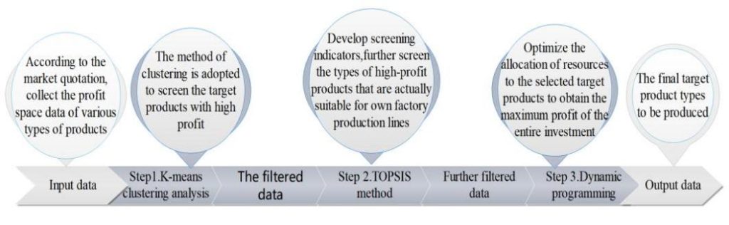
Figure 1. The workflow and functions of the three steps

The market is developing rapidly, and the choice of production investment projects presents diversity and complexity. Manufacturing enterprises not only need to select high-profit target products (multiple target products) suitable for their own production but also need to reasonably allocate limited resources to ultimately obtain the maximum total income of all investment projects. Therefore, it is necessary to find a practical and effective method to carry out project screening and resource allocation, which is divided into the following 3 steps:

Step 1: use the clustering analysis method (K-means) to cluster and screen the products with high net profit in the market (high net profit = retail price – cost).

Step 2: use TOPSIS method combined with the limited actual production conditions of the manufacturing enterprise to optimize the sequence of alternative and ideal solutions for the high-net profit products selected by the first step, and the good and bad solutions are sorted. Further select some ideal target projects. And optimize the allocation of project resources for them in Step 3.

Step 3: use the dynamic programming model to optimize the allocation of resources for several target projects selected in the first two steps to obtain the total maximum profit.

Theoretical analysis and software programming simulation are carried out to determine the effectiveness and feasibility of the scheme. In this process, enterprises need to continuously screen according to their actual production conditions to obtain target investment projects, reasonably allocate limited resources and pursue the maximum profit return of the total investment project. This process achieves the best results through continuous testing and optimization. Finally, enterprises need to evaluate the proposed solutions to determine their actual application effects and make corresponding improvements or adjustments.

Figure 2 shows the entire optimization process of screening and allocation. The series command of MATLAB software will be used to connect the three models in the series to conduct the initial screening of investment production projects, the secondary screening of target investment production projects by combining their own production conditions and the optimal allocation of project resources. The following is the flowchart of the entire working process:

Figure 2. The flowchart of the entire working process

Grammar:

1. series
2. sys = series (sys1, sys2)
3. sys = series (sys1, sys2, outputs1, inputs2)

Description:

Series connect two model objects in a serial fashion. This function accepts any type of model. Both systems are either continuous or discrete and have the same sampling time. Static gain is neutral and can be specified as a regular matrix.

Series 1: Connect the K-means clustering analysis model (sys1) and the TOPSIS method (sys2) in series as follows: sys = series (sys1, sys2, outputs1, inputs2) to form a common series connection (the entire process is shown in Figure 3). Sys1 will filter out dataset d from dataset b and output dataset d to sys2, which will further filter data d and output a new dataset g:

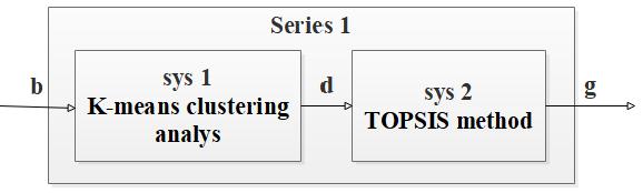
Figure 3. K-means clustering analysis model and TOPSIS method in series

The index vectors outputs1 and inputs2 should connect the output d of sys1 and the input d of sys2.The resulting model sys takes b as input and g as output.

Series 2: Connect the TOPSIS method (sys 2) and dynamic programming (sys 3) in series as follows: sys=series (sys2, sys3, outputs2, inputs3) to form a common series connection (the entire process is shown in Figure 4), sys 2 will further filter data d and output a new dataset g, the new dataset g will be optimized for resource allocation in sys 3 and finally output dataset h to schedule production:

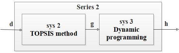
Figure 4. TOPSIS method and dynamic programming model in series

This command is equivalent to direct multiplication: sys = sys2 * sys1

Through the above two-step MATLAB instructions, the three models can be arranged in series, the data can be input and processed in sequence, and finally a project dataset arranged to be produced can be output.

2.1. Step 1 – K-means clustering analysis

Here, the goal of using K-means clustering analysis by manufacturing enterprises (He & Wei, 2024) is to divide the profit data set of various types of products in the market collected roughly in the early stage into K clusters, where one cluster is set to the enterprise’s desired target high profit cluster, and the profit size of each product is equivalent to the length of the Euclidean distance (Al-Ali et al., 2024).

By minimizing the sum of squared distances within the cluster, data points are clustered within the cluster, so that each data point belongs to the nearest cluster center. The cluster center is the average of all points in the cluster, representing the center position of the cluster. The enterprise sets the desired target profit as one cluster center, and by repeatedly adjusting the position of the cluster center, K – means continuously optimizes the tightness within the cluster, thereby obtaining clusters that are as compact and separated as possible and accurately identifying the product types belonging to the target profit cluster, completing the first screening (Zhu, 2024).

The basic process of K-means cluster analysis screening consists of 5 steps, but the process of screening is divided into two main steps: Assignment and Update. Figure 5 shows the process:

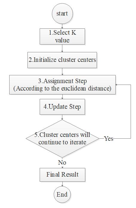
Figure 5. The process of K-means cluster analysis screening

The detailed processes are as follows:

Step 1: Select K value

Set the quantity K of cluster. The quantity of K depends on the target plan of the manufacturing enterprise.

Step 2: Initialize cluster centers

Select K data points as the center of the initial clusters, set an initial target profit data point as an initial cluster center of K clusters (Agbulu et al., 2024).

Step 3: Assignment Step

For each point in the initial profit data set of various types of products in the market collected roughly in the early stage, assign it to the cluster corresponding to the nearest cluster center. The term “distance” is usually used as the Euclidean distance.

• The goal of K-means is to minimize the Within-Cluster Sum of Squares (WCSS), which is the sum of squares of the distance between each point and the center of its cluster (Matlis et al., 2024), as follows:

(1)

Among them:

K is the quantity of clusters.

c is the point set of the i-th cluster.

e is a data point belonging to c.

μ is the center of the i-th cluster.

||e-μ||2 represents the squared Euclidean distance between data point e and cluster center μ.

• K-means uses Euclidean distance to measure the distance between a point and the cluster center, and its formula is as follows:

(2)

Where n is the dimension of the data (Liu et al., 2023).

• Find the nearest cluster center μ_j for each data point:

(3)

Step 4: Update Step

Based on the current cluster allocation, the center of each cluster is recalculated, that is, the mean of all points in the cluster is calculated as the new cluster center:

(4)

Step 5: Repeat steps 3 and 4

The assignment step and update step are repeated until the cluster center no longer changes (converges) or a specified maximum number of iterations is reached (Akshva, 2023).

MATLAB run instructions are as follows:

1	clc
2	clear;
3
4	% main variables
5	dim = n; % (Pattern sample dimension)
6	k = m;   % (There are k clustering centers)
7
8	load(‘testSet.txt’);
9	PM=testSet;% ( Pattern Sample Matrix)
10	N = size(PM,1);
11	figure();
12	subplot(1,n,1);
13	for(e=1:N)
14	plot(PM(e,1),PM(e,n), ‘*r’); % (Draw the original profit data points)
15	hold on
16	end
17	xlabel(‘X’);
18	ylabel(‘Y’);
19	title(Data points before clustering);
20	CC = zeros(k,dim); %(Cluster center matrix, CC (e,:) is the sample vector with initial value e)
21	D = zeros(N,k); %(D (e,μ) is the distance between sample e and cluster center μ)
22	C = cell(1,k); % (Cluster matrix, corresponding to the samples contained in the cluster. In the
23	initial state, the sample set for cluster e (e<k) is [e], and the sample set for cluster k is [k,
24	k+1,… N])
25	for e = 1:k-1
26	C{e} = [e];
27	end
28	C{k} = k:N;
29
30	B = 1:N; % (In the last iteration. Which cluster does the sample belong to. Set the initial
31	value to 1)
32	B(k:N) = k;
33	for e = 1:k
34	CC(e,:) = PM(e,:);
35	end
36
37	while 1
38	change = 0;%(Used to mark whether the classification results have changed or not)
39	% (For each sample e, the distance to k cluster centers is calculated)
40	for e = 1:N
41	for μ = 1:k
42	%          D(e,μ) = eulerDis( PM(e,:), CC(μ,:) );
43	D(e,μ) = sqrt((PM(e,1) – CC(μ,1))^2 + (PM(e,2) – CC(μ,2))^2);
44	end
45	t = find( D(e,:) == min(D(e,:)) ); %(e belongs to class t)
46	if B(e) ~= t % (The last iteration e did not belong to class t)
47	change = 1;
48	% (Remove e from category B(e))
49	t1 = C{B(e)};
50	t2 = find( t1==e );
51	t1(t2) = t1(1);
52	t1 = t1(2:length(t1));
53	C{B(e)} = t1;
54
55	C{t} = [C{t},e]; % (Add e to class t)
56
57	B(e) = t;
58	end
60	end
61
62	if change == 0 %(If the classification result does not change, the iteration stops)
63	break;
64	end
65
66	% (Recalculate the cluster center matrix CC)
67	for e = 1:k
68	CC(e,:) = 0;
69	iclu = C{e};
70	for μ = 1:length(iclu)
71	CC(e,:) = PM( iclu(μ),: )+CC(e,:);
72	end
73	CC(e,:) = CC(e,:)/length(iclu);
74	end
75	end
76	………………………..(if n>2)
77	subplot(1,n,n);
78	plot(CC(:,1),CC(:,n),’o’)
79	hold on
80	for(e=1:N)
81	if(B(1,e)==1)
82	plot(PM(e,1),PM(e,n),’*b’); %(Make a graph of class 1 points)
83	hold on
84	elseif(B(1,e)==2)
85	plot(PM(e,1),PM(e,n), ‘*r’); %(Make a graph of class 2 points)
86	hold on
87	……..                   %……………
88	……..                 %……………
89	……..               %(Make a graph of class m-1 points)
90	else
91	plot(PM(e,1),PM(e,n), ‘*m’); %(Make a graph of class m points)
92	hold on
93	end
94	end
95	xlabel(‘X’);
96	ylabel(‘Y’);
97	title(‘Data points after clustering’);
98
99	for e = 1:k    %(Output sample point labels for each class)
100	str=[‘the ‘num2str(e)’ class contains points: ‘num2str(C{e})“];
101	disp(str);
102	end

2.2. Step 2 – TOPSIS method

This step further screens the product types selected in the first step based on the actual production conditions and capabilities of the enterprise, such as production technology, production techniques, production costs and profits, production capacity and production cycle, etc., and finally selects the products that are truly suitable for the enterprise’s own production. Here, the TOPSIS method is used for secondary screening. TOPSIS (Technique for Order Preference by Similarity to Ideal Solution) is a multi-attribute decision-making method that determines the optimal sorting order by comparing the distance between candidate solutions and ideal solutions (Dayi et al., 2024). A positive ideal solution is the solution that reaches the best value on each attribute, while a negative ideal solution is the solution that reaches the worst value on each attribute. At the same time, in order to determine the distance between the candidate solution and the ideal solution, the Euclidean distance between each candidate solution and the ideal solution is first calculated (Masudin et al., 2024). Then, calculate the positive and negative standardized distances between the candidate solution and the ideal solution. The positive standardized distance reflects the closeness between the candidate solution and the positive ideal solution, while the negative standardized distance reflects the closeness between the candidate solution and the negative ideal solution (Akshya et al., 2024).

The optimal sorting order is the order in which the candidate solution has the shortest distance from the positive ideal solution and the farthest distance from the negative ideal solution. The closer the candidate solution is to the positive ideal solution, the higher its score, and the closer it is to the negative ideal solution, the lower its score (Razdan et al., 2024). This can help decision-makers determine the best alternative solution to achieve the goal of multi-attribute decision-making.

Figure 6 are the basic steps for screening and sorting using TOPSIS method:

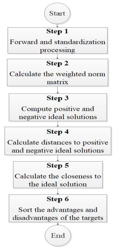
Figure 6. The basic steps for sorting and screening of TOPSIS method

Step 1: Forward and standardization processing.

Through the screening in step 1 (Kumar & Gupta, 2024), assuming there are m evaluation objects (products) selected out by step 1, each evaluation object (product) with n evaluation indicators (production technology, production techniques, production costs and profits, production capacity and production cycle), the original matrix y obtained by comprehensive evaluation is:

(5)

1) Forward processing:

The positive transformation of indicators means that all indicators are transformed into extremely large indicators, that is, the larger the value, the better. In this way, the calculation and code can be more unified and concise (Zournatzidou, 2024).

The types of indicators are: extremely large indicators, extremely small indicators, intermediate indicators, and interval indicators. The conversion method is as follows:

• Extremely small indicators → extremely large indicators.

If all elements are positive, you can also directly take the reciprocal:

(7)

• Intermediate indicators → extremely large indicators.

(8)

Where y_best is the optimal value for this indicator.

• Interval indicators → extremely large indicators.

Among them, a and b are the upper and lower limits of the optimal range of the indicator.

2) Standardization processing

Standardization is carried out to balance the differences or dimensional errors between indicators. There are two methods that can be used (note that if standardization is also performed during forward processing, there is no need for further standardization):

• Z score standardization

(10)

• Map minmax standardization

(11)

The normalized matrix Z is obtained after the forward and standardization processing:

(12)

Step 2: Calculate the weighted norm matrix.

The weight W here can be determined by other methods, such as entropy weight method, etc.

(13)

Step 3: Compute positive and negative ideal solutions.

• Positive ideal solutions:

(14)

• Negative ideal solutions

(15)

Step 4: Calculate distances to positive and negative ideal solutions.

Calculate the Euclidean distance between the target value and the positive or negative ideal solution (Huang et al., 2024).

• The distance from the target to the positive ideal solution is:

(16)

• The distance from the target to the negative ideal solution is:

(17)

Step 5: Calculate the closeness to the ideal solution

(18)

Where 0 ≤ S ≤ 1, when S=0, it indicates that the target is the worst target; When S=1, it indicates that the target is the optimal target. In practical multi-objective decision-making, the possibility of the existence of the optimal and worst targets is very small.

Step 6: Sort the advantages and disadvantages of the targets.

According to the value of Si, the evaluation targets are arranged in ascending order. The larger the S value, the better the target.

MATLAB run instructions are as follows:

1	clc;clear;
2	% y = [y11…….y1n
3	%        y21…….y2n
4	%         …….
5	%          y(m-1)1……..y(m-1)n
6	%              ym1……..ymn ];
7	%
8	% w = [… … … … …]; %“w=Index weight”
9	y = [ .. .
10	.. .
11	.. .
12	.. .];
13
14	%Step1(Data preprocessing – indicator forward)
15	[n,m] = size(y);
16	disp([‘ ‘num2str (n)’ evaluation objects and ‘num2str (m)’ evaluation indicators ‘]);
17	Judge = input([‘ ‘num2str (m)’ indicators need forward processing? Yes, please enter 1. No, enter 0:’]);
18
19	if Judge == 1
20	indicator _label = input([‘ enter the value of each indicator type,such as:extremely large indicators 1/2, extremely small indicators…, intermediate indicators…, and interval indicators… ‘]);
21
22	y = preprocess(y,indicator _label);
23	end
24
25	disp(‘ The matrix after forward processing y =’);
26	disp(y);
27
28
29	%Step1(Data preprocessing – indicator standardization)
30	Z = y./repmat(sum(y.*y).^0.5,n,1);
31	disp(‘ The matrix after standardization processing Z =’);
32	disp(Z);
33
34	%Step2
35	disp(„Quantity of indicators=Quantity of weights (weight sum is 1)“);
36	w = input([‘ Please enter ‘ num2str(m) ‘ weights: ‘]);
37	if abs(sum(w)-1)<0.000001 && size(w,1) ==1 && size(w,2) == m
38	else
39	w = input(‘ If input is incorrect, re-enter the weight row vector:’);
40	end
41
42	%Step3
43	%Step4
44	D_P = sum(w.*(Z-repmat(max(Z),n,1)).^2,2).^0.5;
45	D_N = sum(w.*(Z-repmat(min(Z),n,1)).^2,2).^0.5;
46	% D_P = sum(((Z – repmat(max(Z),n,1)) .^ 2 ) .* repmat(w,n,1) ,2) .^ 0.5;
47	% D_N = sum(((Z – repmat(min(Z),n,1)) .^ 2 ) .* repmat(w,n,1) ,2) .^ 0.5;
48
49	%Step5
50	S = D_P./(D_P+D_N);
51
52	%Step6
53	disp(„The final normalized score and ranking：“);
54	std_S = S./sum(S); % “the final normalized score”
55	[sorted_S,index] = sort(std_S,’descend’)

2.3. Step 3 – Dynamic programming

Dynamic programming is a mathematical method used to solve decision problems with recursive structures, especially those involving sequential decision-making (Barbato et al., 2024). Implementing dynamic programming in MATLAB can be accomplished by defining state variables, decision variables, state transition equations, and objective functions. The following is a specific case analysis. Optimizing project resource allocation for manufacturing enterprises is a very important step.

Assuming that the enterprise runs several target projects selected in the first two steps simultaneously, each project needs to allocate a certain amount of resources, such as funds, personnel, etc., to complete the project (Forghieri et al., 2024). The company’s goal is to maximize the total profit of all projects, and the profit of each project has a non-linear relationship with the amount of resources invested. Resources are limited, therefore dynamic programming is needed to optimize resource allocation. The entire process is shown in Figure 7.

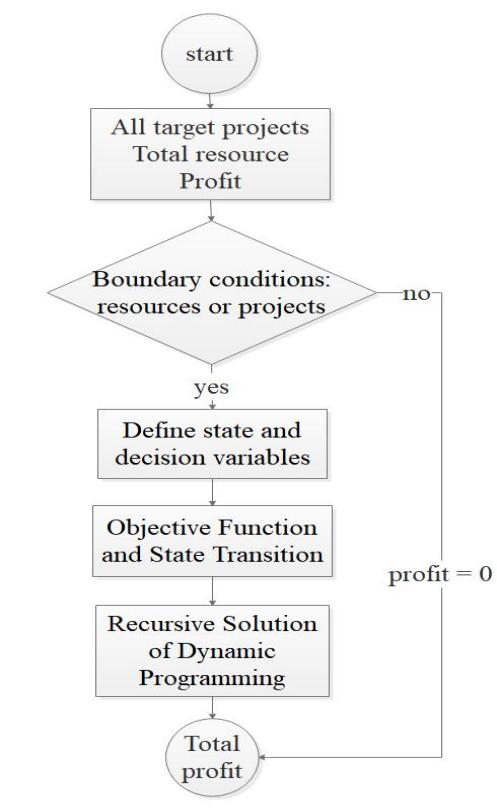
Figure 7. Dynamic programming flow chart

Step 1: Define state and decision variables

• State variable: x (i, j) represents that when processing the i-th project, there are still j units of resources left.
• Decision variable: y (i, j) represents the result of allocating j units of resources to the i-th project.

Step 2: Objective Function and State Transition

• Objective function: Maximize total profit.
• State transition equation:

(19)

Indicate the remaining resources after allocating resources to the i-th project.

Step 3: Recursive Solution of Dynamic Programming

Recursive formula:

(20)

Here, profit (i, t) is the profit obtained from allocating t units of resources to the i-th project.

Step 4: Boundary conditions

When there are no resources or projects,the profit is 0 : Z (0, j)=0 and Z (i, 0)=0.

Step 5: Implement the code

MATLAB run instructions are as follows:

1	function total_profit = resourceAllocationDP(total_resources, profits)
2	n = size(profits, 1);
3	Z = zeros(n + 1, total_resources + 1);  % Initialize DP table%
4
5	%Fill in DP table%
6	for i = 1:n
7	for j = 0:total_resources
8	for t = 0:j
9	Z(i + 1, j + 1) = max(Z(i + 1, j + 1), Z(i, j – t + 1) + profits(i, t + 1));
10	end
11	end
12	end
13
14	total_profit = Z(n + 1, total_resources + 1);
15	end

Through the above calculation process, the limited resources owned by the enterprise are rationally allocated, and the manufacturing enterprise finally obtains the maximum total profit of all projects. This simple and clear process can better help the enterprise to make decisions, avoid the influence of human subjective factors, and achieve objective output results.

The advantage of this screening system is that it uses existing software to calculate the combination of mathematical models and can select target investment projects that are suitable for the production conditions of the manufacturing enterprise from the numerous projects on the market, while optimizing the allocation of project resources and ultimately obtaining the maximum return on investment. The system has the characteristics of pertinence, low cost, simple operation and obvious effect, helping enterprises expand their markets and better adapt to the fiercely competitive market and changing environment.

Conclusions

The combination of K-means clustering analysis, TOPSIS method, and dynamic programming model can effectively solve the problems of inaccurate investment, unreasonable allocation of limited resources, and inability to obtain maximum profit from limited resource investment in the process of selecting production investment projects and allocating limited resources for manufacturing enterprises.

This combination model combines the ability to screen investment projects and optimize limited resource allocation, while also having good profitability. There have been significant improvements and innovations in precision and reliability, which can help manufacturing companies achieve maximum return on investment and the ability to strategically expand their markets. Improve investment decision-making ability, achieve precise and controllable investment, truly combine the limited resources of the enterprise’s own production capacity to obtain maximum returns, and make full use of everything.

However, the combination model also has certain limitations due to the model itself or the connections between models, which are inevitable. For example: the K-means clustering analysis model itself has a significant impact on the selection of initial cluster centers on the final results and can only discover spherical clusters, cannot handle non spherical clusters and is sensitive to outliers.

So, there is no best model, only better models. At present, the development of the manufacturing industry is still plagued by various technological applications and popularization.

However, in the future, with the mature combination and popularization of artificial intelligence technology, the Internet of Things big data and cloud computing, the manufacturing industry will have stronger decision-making, management, scheduling, and profitability capabilities. In the future, our focus will be on the application of high-tech technologies such as artificial intelligence and big data in screening and decision-making systems. However, as the development and maturity of these technologies have not yet reached universality, this is a long process that will be an important challenge for future work.

 

Agbulu, G. P., Kumar, G. J. R., & Gunasekar, S. (2024). IESDCC‑KM: an improved energy-saving distributed cluster–chain K‑communication scheme for smart sensor networks. International Journal of System Assurance Engineering and Management, 15(9), 4443 – 4455. https://doi.org/10.1007/s13198-024-02456-y.

Akshya, K. S., Priyadarsan, P., Muralibabu, K. (2023). Hybrid deep neural network with clustering algorithms for effective gliomas segmentation. International Journal of System Assurance Engineering and Management, 15(3), 964 – 980. https://doi.org/10.1007/s13198-023-02183-w.

Al-Ali, A. S., Haris, R. M., Akbari, Y., Saleh, M., Al-Maadeed, S., Kumar, M. R. (2024). Integrating binary classification and clustering for multi-class dysarthria severity level classification: a two-stage approach. Cluster Computing, 28, 136. https://doi.org/10.1007/s10586-024-04748-1.

Barbato, M., Ceselli, A., Righini, G. (2024). A polynomial-time dynamic programming algorithm for an optimal picking problem in automated warehouses. Journal of Scheduling, 27, 393 – 407. https://doi.org/10.1007/s10951-024-00811-2.

Dayi, F., Cilesiz, A., Yucel, M. (2024). Strategic Management of Clean Energy Investments: Financial Performance Insights by Using BWM-based VIKOR and TOPSIS Methods. International Journal of Energy Economics and Policy, 14(5), 566 – 574. https://doi.org/10.32479/ijeep.16705.

Forghieri, O., Castel, H., Hyon, E., & Pennec, E. L. (2024). Progressive State Space Disaggregation for Infinite Horizon Dynamic Programming. Proceedings of the International Conference on Automated Planning and Scheduling, 34(1), 221 – 229. https://doi.org/10.1609/icaps.v34i1.31479.

He, T., Wei, S. (2024). Hybrid Teaching Platform Design for Ideological and Political Courses Based on K-Means Clustering. In Z. Hou (Ed.). Intelligent Computing Technology and Automation (pp. 660 – 668). https://doi.org/10.3233/ATDE231242.

Huang, S., Cheng, H., Luo, M. (2024). Comparative Study on Barriers of Supply Chain Management MOOCs in China: Online Review Analysis with a Novel TOPSIS-CoCoSo Approach. Journal of Theoretical and Applied Electronic Commerce Research, 19(3), 1793 – 1811. https://doi.org/10.3390/jtaer19030088.

Kumar, M., Gupta, S. K., (2024). Developing a TOPSIS algorithm for Q-rung orthopair Z-numbers with applications in decision making. International Journal of System Assurance Engineering and Management, 15(7), 3117 – 3135. https://doi.org/10.1007/s13198-024-02319-6.

Liu, Y., Zhang, Z., Jiang, S., Ding, Y. (2023). Application of Big Data Technology Combined with Clustering Algorithm in Manufacturing Production Analysis System. Decision Making: Applications in Management and Engineering, 7(1), 237 – 253. https://doi.org/10.31181/dmame712024897

Masudin, I., Habibah, I. Z., Wardana, R. W., Restuputri, D. P., Shariff, S. R. (2024). Enhancing Supplier Selection for Sustainable Raw Materials: A Comprehensive Analysis Using Analytical Network Process (ANP) and TOPSIS Methods. Logistics, 8(3), 74. https://doi.org/10.3390/logistics8030074.

Matlis, G., Dimokas, N., Karvelis, P. (2024). Unveiling University Groupings: A Clustering Analysis for Academic Rankings. Data, 9(5), 67. https://doi.org/10.3390/data9050067.

Razdan, M. R., Aghasi, S., Davoodi, S. M. R. (2024). Ranking Factors Affecting Supply Chain Risk with a Combined Approach of Neutrosophic Analytical Hierarchy Process and TOPSIS. Journal of Applied Research on Industrial Engineering, 11(3), 423 – 435. https://doi.org/10.22105/jarie.2021.303869.1379.

Zhu, Y. (2024). Behavior Analysis of Learner Based on Big Data and Improved K-Means Algorithm. In Z. Hou (Ed.). Intelligent Computing Technology and Automation (pp. 539 – 547) DOI: 10.3233/ATDE231228

Zournatzidou, G. (2024). Evaluating Executives and Non-Executives Impact toward ESG Performance in Banking Sector: An Entropy Weight and TOPSIS Method. Administrative Sciences, 14(10), 255. https://doi.org/10.3390/admsci14100255.